anova

EEG and MEG studies are most often analyzed with a special kind of analysis of variance, that accounts also for within subject changes rather than only for between subject differences. EMEGS offers the possibility to calculate this kind of analysis directly, without exporting the data to a separate statistic software package. Moreover, you can choose between a region-of-interest analysis, averaging over sensorgroups and time points, or a complete analysis for every sensor and time point in your data.

To run a repeated measures ANOVA, prepare your data as described:

Each condition for every subject has to be saved as an SCADS average file. Every file has to have the same number of points and number of channels and the same baseline calculation. You need a textfile, listing the paths of those files on your machine (a 'batchfile'), with one path per line.This batchfile has to reflect the design of the planned analysis, that is, your paths have to be listed according to the hierarchy of your factors. The lowest level is always the subject factor, so you 'll start with one cell for which all subjects average files are given. Beneath that, you list all subjects average files for the next cell etc. The subject order has to be identical in every cell, and you have to have equal number of subjects in every cell. Please note that the structure of the batchfile is identical, wether or not you have defined one or more between factor(s)!!!!!

Unequal cell sizes (between) or missing data (within) are not supported for the matlab-based ANOVA. The R-based ANOVA however supports unequal between cell sizes, and the R-based Mixed-Effect-Models supports both, unequal cell sizes and missing data.

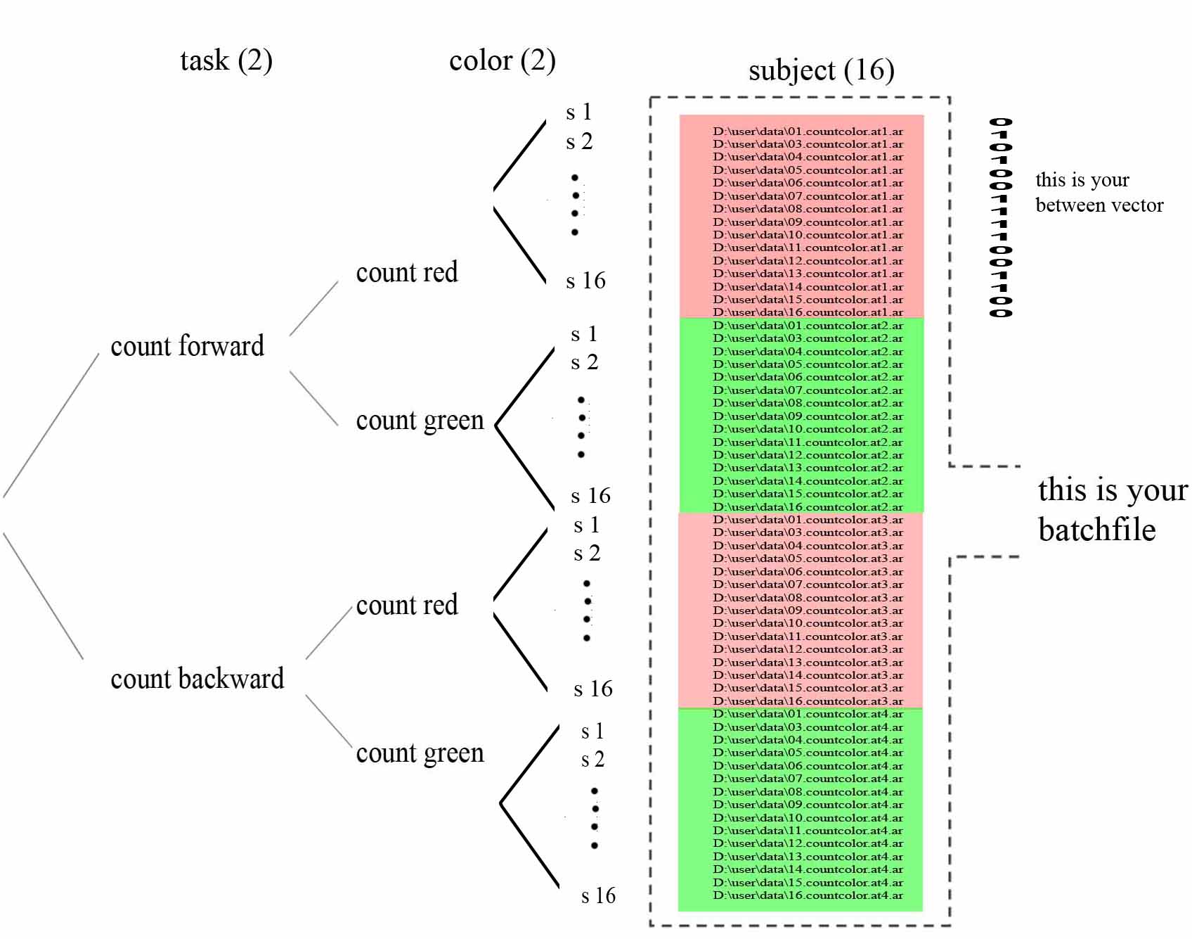
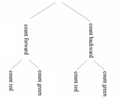
Cells are ordered from lowest hierarchy position of the factor to highest hierarchy position. For instance, consider a 2X2X2 design with the factors 'task' (count forward vs count backward) , 'color' (count red squares vs. count green squares) and 'gender'. Your batchfile for 16 subjects has to have the following form:

The design string would be the following: nrofsubjects: 16; nrofintervalls: 1; nrofchannelgroups: 1; task:2;countforward,countbackward; color:2;countredsquares,countgreensquares; between gender:2;male,female; [0,1,0,1,0,0,1,1,1,1,0,0,1,1,0,0];

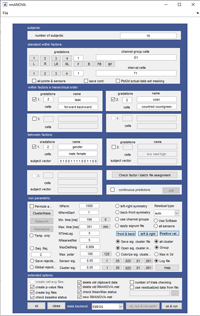
Once you've prepared this, load one of the listed files in Emegs2d, set the baseline and display all points. Start Emegs3d. Here, load the batchfile as filematrix  (File\FileMatrix\LoadBatchfile). Then choose \Calculate\Repeated Measures Anova\Define, pick your preferred input mode (text or gui (graphical user interface) ), and enter your design. The GUI-way is mostly self-explanatory, for the text mode, you can follow the example above. With either mode, you always have to enter the following three parts: number of subjects in your sample (ignoring betweenfactors, that is the total number subjects in all groups), the number of channelgroups and the number of intervalls using the following syntax:

All other within factor definitions are optional and have to comply with the following syntax:

Between/group factor definitions have the following syntax:

As you can see, one difference to the within factors is the subject vector, which specifies the group affiliation of each subject ( in text-mode, this vector forms a new line right after the factor declaration ). You can supply any integer numbers as group indices, but no strings. These numbers are mapped to the cell names according to their value: the lowest number will be the first group, the next higher number the second group etc. . Subject vectors have to have one element for each subject, but subjects do not have to be grouped according to their group membership (a vector like [0 0 1 1] is equivalent to [0 1 0 1] if your batchfile is ordered accordingly. The second difference to a within factor definition is the mandatory keyword 'between' before the actual factor definition.
If you whish to calculate the design for all points and channels and view the output as SCADS average files, set nrofintervalls to the total number of points in your data files and nrofchannelgroups to the number of channels (text) or check the 'all points and channels' checkbutton (gui). Please note, that with a high number of channels and timepoints, this analysis quickly exceeds the available RAM of your computer. To effectively avoid the crash, you can reduce the spatial and temporal resolution by using 'Intervall means' and/or 'channelgroups' (see below).
If you want to run one special analysis across a selected number of channels and certain time points, enter the number of channelgroups and the number of timeintervalls correspondingly. These values have to match the channelgroups loaded in Emegs2d and the time/intervall settings in Emegs3d. If more than one of each is provided, channelgroup and/or time will be a separat factor in the ANOVA. Please not that for a true pointwise analysis, the whole intervall has to be selected in Emegs3d including the baseline points!!!
If you want to use channelgroups and/or intervalls (using Emegs2d\Calculate\Channelgroups and Emegs2d\Calculate\Intervall Mean) but still want the output as continuous SCADS-files, add the line 'continuous results;' at the end of the design (text) / check the 'continuous results'-checkbox (gui). The result files will be stepfunctions of time: all timepoints in a defined intervall will have the same value. This is also true for channelgroups: all sensors in a channelgroup will have the identical stepfuntions. Intervall and channelgroup definition files can either be created and loaded manually or automatically by using the 'Auto intervalls' or 'Auto groups' menuitems. The automatic creation usually is much easier and sufficient in the case, that you only wish to use intervalls/channelgroups to reduce memory load.
Click 'OK' and choose \Calculate\Repeated Measures Anova\Run Anova or click the 'OK & Run'-button. For a pointwise/continuous analysis, you will be prompted for a target folder, where results are going to be saved. EMEGS will save two average file in SCADS format for every factor and interation in your ANOVA, one with p-values, one with the F-Values. For a single analysis results will be displayed in new figure, from which you can calculate post-hoc test, display means graphically and export the data to a text file.

Post-Hoc Contrasts: Post-Hoc Contrasts usually are calculated for significant effects found in an analysis of variance. In EMEGS this can be done for one specific analysis of interest and also for every sensor and time point. Post-Hocs for one analysis of interest can be calculated from the output window displaying the ANOVA-results. It requires that you first start the plotting mode by choosing '\Graph\Cellplot' in this window and then plot the effect that you wish to explore, by adding it's components to the plot on the anova-plotting menu (see below). Then you can compare all cells by choosing '\PostHoc\Entire family' (without alpha-error correction). Alternatively, you can enter specific coefficients for your cells by choosing '\PostHoc\Custom contrast'. Moreover you can calculate a series of contrasts using the Bonferroni-Holm stepdown procedure for alpha-correction by choosing '\PostHoc\Bonferroni Holm'. For this, you need to create a contrast text-file, containing your coefficients for every contrast to calculate with one contrast per line. EMEGS then calculates these contrasts, sorts them by their significance level, and tells you which ones can be considered significant. Results of all the described tests are appended to the anova results in the listbox of the results window.

To calculate Post-Hocs for every sensor and time point, choose \Emegs3d\Calculate\Repeated measures anova\Pointwise post-hocs'. A window will open, that lets you select an effect or interaction to be explored. When you`re done selecting your effect, hit the 'Calculate post-hocs'-button. EMEGS will then create one average file for all possible cell comparisons in the selected effect (for the entire family), containing the uncorrected p-values of the corresponding contrasts and name the resulting files using the cell labels specified in the anova design.

Exporting data to an external statistics software: To analyse your data in a methodically more sophisticated fashion, e.g. to correct for violations of variance homogenity or other assumptions or to calculate certain types of post-hoc contrasts, it is often necessary to export your data to a dedicated statistic software. The ANOVA-plotting module offers a way to export the current data matrix in a text-file, that can easily be read by SPSS, Statistica, Jump or other packages. To do this, choose \data\export data from the figure showing your ANOVA results. You will be asked to choose a decimal separator and a filename and filelocation. Variable lables of  grouping factors are taken directly from your design. Columns for repeated measurements however are labelled using the following pattern: 'c' stands for channelgroup, 't' for time/intervall and 'm' codes the product of all other custom within factors. Columns are ordered according to the hierarchy of the factors. Thus, the export for the above example looks something like this:

As in the example the time factor is limited to 1 intervall and only one channelgroup is used, there are only 4 columns corresponding the cells of the 'task' and the 'color' factor with 2 gradataions (2*2 = 4 total) each. This arrangement of the data is in line with the way SPSS and Statistica are calculating ANOVAs with repeated measurements and corresponds the transposed structure of the batchfile we used for calculating the ANOVA.

subject	gender	m1c1t1	m2c1t1	m3c1t1	m4c1t1
1 2 3 . . .	0    1    0    . . .	-3,1144    -9,4074    -1,6262    . . .	-0,51314 2,1428    -5,1445    . . .	-1,6344    -2,4501    1,9558    . . .	2,1613    2,1346    2,6973    . . .