Command: Plugtfwltgui.
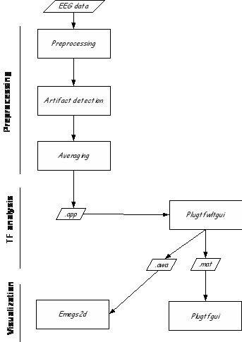
In addition to the standard Emegs toolbox (WaveApp), the plugins Plugtfwltgui and Plugtfgui offer integration with the fieldtrip toolbox (http://fieldtrip.fcdonders.nl/), to run wavelet-based time frequency analysis.
The Fieldtrip toolbox is documented elsewhere (see http://fieldtrip.fcdonders.nl/tutorial/timefrequencyanalysis ; see also Roach & Mathalon, 2008 for a comprehensive review on time-frequency analysis). In the following, the Emegs interface for time-frequency analysis using fieldtrip will be described.
To use this plugin, you need to have a recent version of eeglab installed (http://sccn.ucsd.edu/eeglab/). Eeglab includes fieldtrip, so no further software should be required. This plugin has been developed/tested with eeglab 7.2.9.19b .
The initial analysis steps (preprocessing, artifact detection, averaging) are documented elsewhere. After averaging, single trial EEG files are created (.app files), which will be used to run time-frequency analysis.
First, you need to create a batchfile of all the app files you want to analyze. You can do this either manually, by using a command-line program (e.g. dir2batch) or by using the emegs file manager.
When the batchfile is created, you can open the analysis plugin (plugtfwltgui) either by entering the command plugtfwltgui, or by selecting ' run fieldtrip TF analysis' in the Plugin menu of Emegs2d.
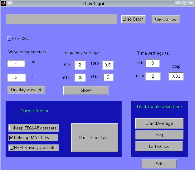
The plugin interface allows you to:
run the analysis either on average referenced or on CSD data;
vary wavelet parameters
use variable frequency resolution
export to eeglab
export to emegs
operate on fieldtrip files (grandaverage, average, difference)
CSD. It has been suggested that, to avoid signal contamination by spatially remote sources, a CSD reference is used. This can be done by selecting 'Use CSD'. If this is unchecked, the reference chosen in the preprocessing steps is used.
Wavelet parameters. Wavelets (more specifically, Morlet wavelets) vary in two important temporal properties: the number of wavelet cycles (m), and the temporal standard deviation of the wavelet itself (c). These parameters are described elsewhere (e.g., Roach and Mathalon, 2008), and can be set by entering the m and c values under 'wavelet parameters'. Clicking on 'display wavelet', a diagnostic plot is displayed. In the upper row, the wavelet fro the lowest and highest frequency band are displayed.
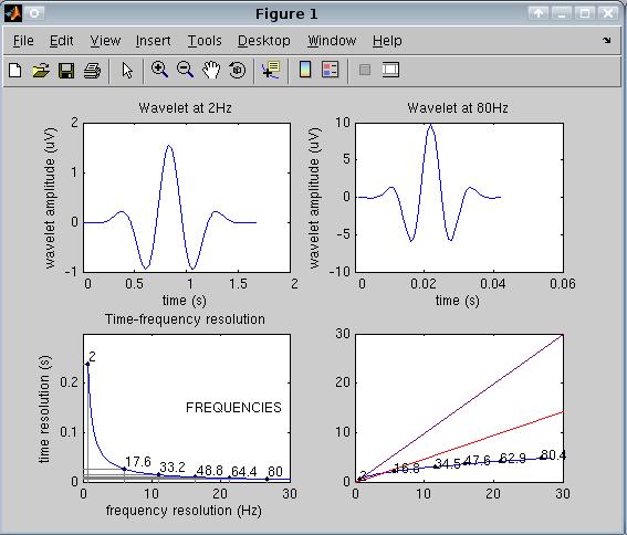
Choosing appropriate m and c values is essential to achieve sufficient temporal and frequency resolution in the analysis. Time and frequency resolution is shown in the bottom left plot.
Variable frequency resolution. This interface allows to choose a variable frequency resolution for low and high frequencies. Time-frequency analysis can only achieve good time OR frequency resolution, but not both. At low frequencies, time resolution is bad but frequency resolution is good (that is, you can distinguish between two neighboring frequencies, but not between two time points if these are very close), while the opposite happens at high frequencies (good time but bad frequency resolution). For this reason, the interface allows to choose a small frequency step for low frequencies, where frequency resolution is good, which increases towards a large frequency step for high frequencies, where frequency resolution is bad. For instance, setting analysis from 2 to 80 Hz, a minimum step of 0.5 and a maximum step of 5 Hz, you will analyze the following frequencies (you can see this plot by clicking 'show' below 'frequency settings':

In the left panel, frequency step is displayed as a function of frequency, and ranges from 0.5 (at 2 Hz) to 5 (at 80 Hz). Using 30 steps, the entire 78 Hz interval is analyzed. In the right panel, an horizontal grid shows the frequency coverage , with more dense steps in the lower compared to the higher frequency ranges.
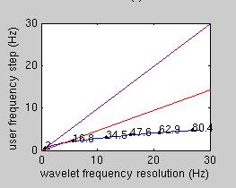
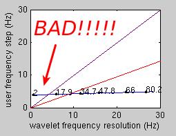
The lower-right panel in the first diagnostic plot in the 'display wavelet' plot compares the chosen frequency step to the wavelet frequency resolution. On the x axis, the wavelet frequency resolution is displayed. These values depend on the chosen m and c parameters. The purple and the red lines display the hypothetical situation where the user selects frequency steps which are the same (purple) or half (red) of the wavelet frequency resolution. As a rule of thumb, the blue line should be below the red line. If the blue line is above the red or (worse) the purple line, then you have chosen a frequency step which is larger than the wavelet frequency resolution, and your analysis is prone to miss important effects which are in the data.
Temporal settings. You can set the beginning and the end of the epoch to analyze. Enter numbers in seconds, relative to the beginning of the epoch (i.e., 0 is the first point in the epoch). Also enter a temporal step between successive time points. In choosing this value, keep in mind the temporal resolution of your wavelet!
Output format. By default, Plugtfwltgui saves a matlab file (.mat) containing two fieldtrip data structures: pwr for power data, and phs for phase-locking factor. Additionally, you can export data to the standard emegs format for wavelet data (awa and pwa files), by checking 'EMEGS awa/pwa files'.
To run the analysis, a temporary eeglab file containing the single trial EEG information (NOT the results of the time-frequency analysis) is created. This file is normally deleted, however you can ask to keep this data file by checking 'Keep EEGLAB datasets'.
Done! You can click on 'Run TF analysis' and let it run. Depending on the amount of data, computing power, etc., it may take some time (usually a lot). You can even run into memory problems, so you might want to reduce the data to analyze. If everything works, after some time you will get one .mat file for each of the .app files you asked to analyze.
Fieldtrip file operations. After you have the .mat files, you can create grandaverages, or perform simple operations on individual mat files.
Grandaveraging requires you to have your data organized by folders (one folder for each participant). Click on grandaverage and create a dummy-file (e.g., aaa) in the top-level folder (the one containing the participant subfolders). It will scan your data, understand how many conditions you have, average similar conditions together, and put the grandaverage files in the top-level folder.
Avg asks you for some files, which will be averaged together.
Difference asks you for two files, which will be subtracted one from the other.
When this is done, use plugtfgui to display the results, and to export data as text files.