filtering and segmentation
Commands: PrePro, FilterNetFile,
FiltNeuroscanFiles, FiltBdfFiles, TransNetGeoHist,
NeuroScanToEgis, TransMsiContSess, CalcAutoEditMat, CalcAutoEditMEGMat,
TransRawTaw, TransBdfBdt, emesgsreadbdfmarker
Filtering and segmentation can be done manually, using scripts like Batch.m' that call 'FilterNetFile', or, or by using 'PrePro' user
interface.
Filtering and
segmentation using
PrePro
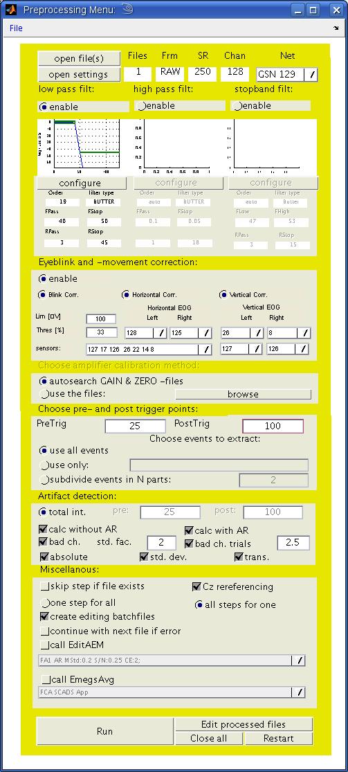
PrePro, when started, is disabled, and waits for you to open a
data file, or to load a batchfile containing paths of datafiles.
Datafiles must have the same format (EGI, EGI (E1), Neuroscan,BDF, EDF
or BTI) and the
same sampling rate and the same number of channels. After succesfully
loading a file, the number of channels and the sampling rate are
displayed in the upper right corner. For EGI sensor configurations,
there are predefined eye movement and -blink sensor configurations that
can be selected from the 'Net' dropdown box. PrePro selects the proper
sensor net automatically, if your raw data file names contain the
keywords '.GSN.' and '.HC1.' for old style geodesic sensor nets or
hydro-cell sensor nets respectively. For instance the datafile with 129
channels 'Test01.GSN.RAW' will be automatically selected for Net "GSN
129", and VEOG/HEOG and blink sensors will be set accordingly.
 Filters:
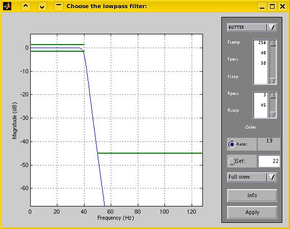
After
loading a file, you can activate and configure highpass, lowpass and
stopband filters by enabling their radio-buttons. Initially you have to
configure every filter, that you enable. An example of the filter
configure dialog is given below (click to enlarge). The graph displays
the attenuation of the signal (blue line) caused by the filter in
dezibel for the range of frequencies. The default setting for a
lowpass-filter as in the example below, consists of an attentuation of
the stopband (frequencies above 50 Hz) of at least 45 dB (which means
that amplitudes are a not greater than the ten-thousandth part of their
original values), and a negligable attenuation of the passband
(frequencies below 40 Hz; amplitudes decrease not below about three
fourths of their original value). The desired stopband and passband
attenuation are displayed as green lines, and can be changed, just as
the cut-off frequencies, to design other filters. Similar filter
design dialogs are available for highpass and stopband
filters.
Filters:
After
loading a file, you can activate and configure highpass, lowpass and
stopband filters by enabling their radio-buttons. Initially you have to
configure every filter, that you enable. An example of the filter
configure dialog is given below (click to enlarge). The graph displays
the attenuation of the signal (blue line) caused by the filter in
dezibel for the range of frequencies. The default setting for a
lowpass-filter as in the example below, consists of an attentuation of
the stopband (frequencies above 50 Hz) of at least 45 dB (which means
that amplitudes are a not greater than the ten-thousandth part of their
original values), and a negligable attenuation of the passband
(frequencies below 40 Hz; amplitudes decrease not below about three
fourths of their original value). The desired stopband and passband
attenuation are displayed as green lines, and can be changed, just as
the cut-off frequencies, to design other filters. Similar filter
design dialogs are available for highpass and stopband
filters.
Eyeblink and -movement correction: When activated, this
module offers you the choice of three separate submodules, the blink
correction, the horizontal eyemovement correction and the vertical
eyemovement correction. All three are based on the algorithm proposed
by Gratton, Coles and Donchin (1982). At
the present stage, this algorithm is tested only for EGI data,
and the default sensors chosen as Blinksensors, VEOG-sensors and
HEOG-sensors are only correct for EGI systems!!!!
To run the blink correction, you have to create a mat-file, containing
a typical blink ( a 'blinkfile') for every datafile you are analyzing before you can start the
preprocessing. This is done in emegs2d, using the
'EgisContinuous'-dataformat (again this option is only available for
EGI data so far). Select this dataformat from the menu \file\data
format\Egis Continuous and open a *.RAW-file using the 'Open
Dataset'-button. EMEGS then searches for the corresponding *.ZERO- ,
*.GAIN- and *.HIST-files and reads their content to display calibrated
amplitudes and trigger events. Once the continuous data is displayed,
click the 'mouse'-button on the emegs2d-menu and leftclick on the
datawindow. A grey surface will appear. Scroll to a typical blink using
the cursor point slider and move the grey surface symmetrically over
the blink. You can either drag it, or recreate it in a propper
position, by leftclicking at the start point ( has to be outside the
surface ), and dragging the mouse to its desired end point. The center
of the surface will be taken as blink maximum in the correction
algorithm, therefore it is important to make the selection symmetrical
to the blink peak. Then rightclick on the grey surface (preferably at
the top of the datawindow to avoid other objects under the mouse) and
select 'write blinkfile'. You are then prompted with a butterfly-plot
of the blink, to allow you to check your chosen intervall. Select 'ok'
and accept the suggested name for the blink file (corresponding the
*.RAW-filename with the *.blk-extension). If you give it a different
name or choose to save it in a different folder than the folder
containing the *.RAW-file, EMEGS will not find it later on!!!
The correction is done on data epochs stored in the E1-file, to
allow subtraction of the event-related EOG before correction (see the
Gratten & Coles paper). If you wish to compare the non-corrected
and the corrected trials, open
the E1.original-file and the E1-file using the Egis session-dataformat in emegs2d,
and select the trials listed in the >>*E1.Blinktrials.txt
<< (these are the trials which blinks were found in).
Amplifier
calibration: This options is only available for EGI data.
Neuroscan data is analyzed presuming all GAINS to be 1 and all ZEROS to
be , BDF amplifier calibration is read from the data file. For
EGI-data, you can one specific set of GAIN and ZEROs, that
will be used for all files, or have PrePro search for a GAIN and ZERO
for every data file in the batch separately. This is done simply by
using the filename, so be sure, to have consistent filenaming.
Segmentation: By
entering numbers in the PreTrig and PostTrig boxes, you can define how
many points will be taken before each event and how many after. Events: The default behaviour
in PrePro segmets your data for every kind of event it encounters. If
you do not like this, you can activate the 'use only'-box and enter
numbers, corresponding the trigger values that you wish to use. All
others will be ignored. If you want to subdivide events into
halfs/thirds/fourths etc, check the 'subdivide event'radiobutton and
enter the desired denominator.
Artifact
detection: PrePro automatically chooses
the entire extracted intervall, to calculate statistical parameters,
that afterwards are used for artifact detection. If you wish to use
only a certain part of the intervall for this purpose, you can define
separate PreTrig- and PostTrig-points for artifact detection. Generally
a longer intervall is more likely to contain artifacts, thus leading to
less good trials.
Miscellaneous: The option 'skip step if
file exists' lets you avoid repeating one step if it already has been
performed and procuded a result file. This can save you time, but will
cause a crash in the case that an incomplete or corrupted file
exists. 'One step for all' vs. 'All
steps for one' refers only to batch processing, and specifies wether
PrePro will perform one step (for instance the segmentation) for
all files in the batch before going one with the next step. Otherwise,
all steps will be performed for one file, and then all steps for the
next etc. The latter is generelly preferable for long batches, that you
do not want to crash half way through. Thus, if a problem occurs on one
file, PrePro will still get the other files right, assuming that you
checked the 'continue with next file if error'-option. This
latter option makes only sense for batch processing and works more
specifically only for the 'all steps for one'-type. In this case, if an
error occurs on one file, PrePro jumps to the next file in the batch.
All settings including the filematrix can be saved and loaded using the
menu \File\Default File.
Manual filtering and segmentation
Manual preprocessing using a custom script or using the command
line can be done as shown in the file 'Batch.m'.
This is intended to be a standard preprocessing
script, that you can adopt to your specific demands.
Generally, filtering a
raw-data-file saves the filtered data in a new
file, adding filter-dependant characters to the filename. A lowpass
40Hz filter, for instance, transform the file '01.run1.taw' to 01.run1.fl40.taw'.
To filter data files, you can use the scripts 'GetLowFiltCoeff',
GetHighFiltCoeff', 'GetHighLowFiltCoeff' and 'GetStopFiltCoeff' to
design the filters and then use 'FilterNetFile', 'FiltNeuroscanFiles',
FiltTransNeuroscanFiles' and 'FilterStopNetFile' to do the actual
filtering.
To cut continuous data files into trials, use 'TransNetGeoHist'
(EGI-format), 'NeuroscanToEgis' (Neuroscan-format) or TransMsiContSess
(BTI-format). The trials will be saved in an *.E1-file (EGI) or in a
*.ses-file (Neuroscan & BTI). Trigger information will be written
in a *.CON file (for all formats).
File
types
EGI Format: EGI data files have to be exported using the
netstation software, so you end up with a set of 5 files per run (*.RAW,*.HIST,*.ZERO,*.GAIN,*.IMP).
The RAW-file is then transformed (pointwise sorting is
tranformed to channelwise sorting) into a TAW-file that
contains the same data. This file in turn is used for filtering,
resulting in a modified TAW-file, for instance *.fl40.TAW
for a 40Hz lowpass filtering.
During segmentation in 'TransNetGeoHist' the trials are saved in an *.E1
file, containing all trials including artifacts and broken channels. A *.CON
file is generated containing the trigger information for each trial.
Statistical parameters used for artifact correction and calculated in
'CalcAutoEditMat' are saved in an *.AEM and an *.AEM.AR-file
(AEM signifies Auto-Edit-Matrix, AR stands for average reference), flat
or corrupted sensors are listed in a *.Xest-file (with X
replaced by your number of channels). Editing the data using 'EditAEM'
creates two new files: a *.WE-file and a *.TVM-file, both
containing good and bad trials and channels. During averaging using
'EmegsAVG', bad sensors in the trials from the *.E1-files are
interpolated and trials are averaged based an the *.WE-files,
your sensor configuration file (*.ecfg), and the *.CON
file, resulting in a set of 3 files for each condition: an *.APPx-file,
containing only good and approximated trials of the condition x, a
corresponding *.ix file, listing the indices of the good trials
for this condition, and an *.atx file, containing the averaged
waveform.
Neuroscan Format: Neuroscan *.cnt data files have to be
filtered using 'FiltNeuroscanFiles', resulting in a modified cnt-file,
for instance *.f.cnt.
During segmentation in 'Neuroscan2Egis' the trials are saved in an *.ses
file, containing all trials including artifacts and broken channels. A *.CON
file is generated containing the trigger information for each trial.
Statistical parameters used for artifact correction and calculated in
'CalcAutoEditMat' are saved in an *.AEM and an *.AEM.AR-file
(AEM signifies Auto-Edit-Matrix, AR stands for average reference), flat
or corrupted sensors are listed in a *.Xest-file (with X
replaced by your number of channels). Editing the data using 'EditAEM'
creates two new files: a *.WE-file and a *.TVM-file, both
containing good and bad trials and channels. During averaging using
'EmegsAVG', bad sensors in the trials from the *.ses-files are
interpolated and trials are averaged based an the *.WE-files,
your sensor configuration file (*.ecfg), and the *.CON
file, resulting in a set of 3 files for each condition: an *.APPx-file,
containing only good and approximated trials of the condition x, a
corresponding *.ix file, listing the indices of the good trials
for this condition, and an *.atx file, containing the averaged
waveform.
BDF Format:
From the raw BDF-file, the status channel is initially analyzed for
non-zero values. These values are written with there begin and end time
to a *.HIST file, that is
later used for extracting data epochs. The raw BDF-file is
transformed (recordwise sorting is
tranformed to channelwise sorting) into a BDT-file that
contains the same data. This file in turn is used for filtering,
resulting in a modified BDT-file,
*.f.BDT after filtering.
During segmentation in 'Bdf2Egis' the trials are saved in an *.ses
file, containing all trials including artifacts and broken channels. A *.CON
file is generated containing the trigger information for each trial.
Statistical parameters used for artifact correction and calculated in
'CalcAutoEditMat' are saved in an *.AEM and an *.AEM.AR-file
(AEM signifies Auto-Edit-Matrix, AR stands for average reference), flat
or corrupted sensors are listed in a *.Xest-file (with X
replaced by your number of channels). Editing the data using 'EditAEM'
creates two new files: a *.WE-file and a *.TVM-file, both
containing good and bad trials and channels. During averaging using
'EmegsAVG', bad sensors in the trials from the *.ses-files are
interpolated and trials are averaged based an the *.WE-files,
your sensor configuration file (*.ecfg), and the *.CON
file, resulting in a set of 3 files for each condition: an *.APPx-file,
containing only good and approximated trials of the condition x, a
corresponding *.ix file, listing the indices of the good trials
for this condition, and an *.atx file, containing the averaged
waveform.
BTI Format: BTI data files, at the present stage, have to be
noisecorrected, cardiaccorrected and filtered externally. EMEGS scripts
for this are not yet available.
During segmentation in 'TransMsiContSess', the trials are saved in a *.ses
file. A *.CON file is generated containing the trigger
information for each trial.
Statistical parameters used for artifact correction and calculated in
'CalcAutoEditMEGMat' are saved in an *.AEM -file (AEM signifies
Auto-Edit-Matrix). Editing the data using 'EditAEM' creates the *.WE-file,
containing good and bad trials and channels. During averaging using
'EmegsAVG', bad sensors in the trials from the *.ses-files are
interpolated and trials are averaged based an the *.WE-files,
your sensor configuration file (*.ecfg), and the *.CON
file, resulting in a set of 3 files for each condition: an *.APPx-file,
containing only good and approximated trials of the condition x, a
corresponding *.ix file, listing the indices of the good trials
for this condition, and an *.atx file, containing the averaged
waveform.
References:
Gratton, G., Coles, M.G.H. & Donchin, E. (1982). A new method
for
off-line removal of ocular artifact. Electroencephalography and
clinical Neurophysiology, 1983, 55: 468-484.