Commands: ReadEConfig,
SaveEConfig
sensor
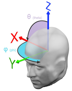
coordinates: Sensor positions im emegs are
defined as spherical coordinates. These are given as two angles, theta
and phi that are measured from the upward (z) axes as shown in the
graph below. Note that this does not correspond the MATLAB definition
of spherical coordinates, therefore standard MATLAB coordinate
conversions (sph2cart or cart2sph) will not work. Use change_sphere_cart instead.
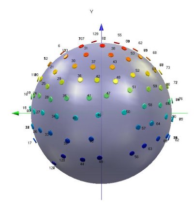
You can display a loaded sensor
configuration using the command \View\View
sensor config from
emegs2d-menu. The picture below shows a EGI 129 channels sensor configuration.
sensor
configuration files: Sensor configuration files
in emegs are binary files ( use the functions ReadEConfig and SaveEConfig to read and save this
file type), stored in the
folder \emegs2.1\emegs2dUtil\SensorCfg\.
To determine
which of these configuration files to load, emegs
looks up a list of configuration file, stored in the textfile \emegs2.1\emegs2dUtil\ViewDefault\DefaultEcfg.txt
and takes from this list
the first filename, that contains the
needed number of channels in the
filename. Thus if a configuration file for 129 channels is
needed, and the DefaultEcfg.txt-file contains the following:
then emegs will load the file \emegs2.1\emegs2dUtil\SensorCfg\
129.ecfg to display the data. This file would also
be taken, if the entry would be named SConfig129.ecfg
or 129XXXX.ecfg, as long as
the number of channels is found in the filename. For the standard planar display of a
multichannel sensor array, these positions are projected on a plane
using the transformation:
where EPosSpher is a NChannels X 2 -Vector
containing the Theta angle in the first column, and the Phi
angle in the second column.
sensor configuration dependant leadfield coefficients: the calculation of spherical spline interpolations (used in artefact editing and 3d plotting), laplacians, cortical Maps and l2-min.-norms (used for source localization) depend on leadfield calculations, which again depend on your sensor configuration. In order to minimize calculation time emegs3d saves calculated leadfield coefficients in the emegs3dCoeff40 as well as emegs3dInvCoeff folder. Prior leadfield calculation emegs3d checks for possibly existing coefficient files for the particular sensor configuration in these folders and reads them in, instead of calculating them again. Therefore, you must not name different sensor configurations identically. The program would use the original existing (now wrong) coefficients, as it is not able to check if the sensor configuration were changed. In case you would like to keep sensor configuration names and change the configuration you have to delete all corresponding leadfield coefficient files in the folders mentioned above. Leadfield coefficient file names contain the configuration names e.g Scalp_129_32_15 corresponds to the sensor configuration 129.ecfg. The files DLoc_*.* in folder Emegs3dInvCoeff contain the inverse leadfield dipole positions and must not be deleted.