 Actual dipole (like actual data set
in Emegs2d menu)
Actual dipole (like actual data set
in Emegs2d menu) Command: GenSynthData
Opens
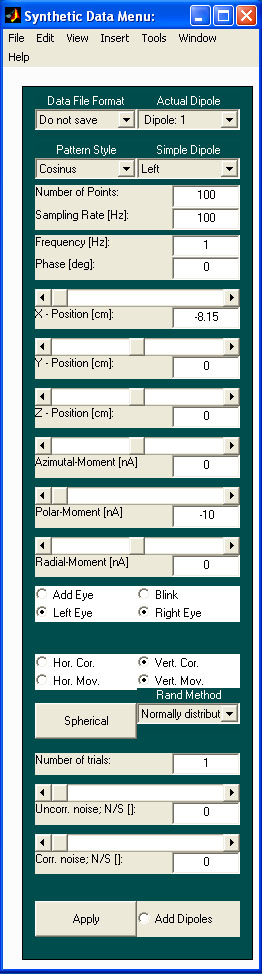
a new menu figure named: Synthetic data menu (calls GenSynthData.m)
Actual dipole (like actual data set
in Emegs2d menu)
All changes of position, moments etc. concerns to this chosen dipole.
To get an additional dipole choose More.
The default position is [0 4 6]. The default dipole moment is [0 0 1].
To reject the last dipole choose Less.
The synthetic menu starts with two default dipoles of 100 points of time:
Dipole 1: Position [-4 0 6] and the cartesian dipole moment [0 1 0]. The default pattern is of Cosinus style with a frquency of 1 and a phase shift of zero.
Dipole 2: Position [+4 0 6] and the
cartesian dipole moment [0 1 0]. The default pattern is of Sinus style
with a frquency of 1 and a phase shift of zero.
X direction from left ear to right ear
Y direction from posterior to anterior
Z direction from inferior to superior
You could change position, moments of the actual dipole using the position text or slider menus.
The program double checks whether the chosen dipole position lays into the given sphere with an radius of 8.15 cm. Otherwise the old position would be taken.
The dipole moments could be chosen between �1 and 1 for each direction.
If spherical coordinates are chosen the polar angle is the one from inferior to superior (-1 from superior to inferior)
The positive azimutal angle shows counterclockwise looking from top to the x-y plane.
(if the position is right ear the moment shows from posterior to anterior)
(if the position is the nasion the moment shows from right to left)
(if the position is left ear the moment shows from anterior to posterior)
(if the position is the inion the moment shows from left to right)
Pattern Style:
Linear: The pattern (time course) of the actual dipole strength is constant (1) across time.
Cosinus: The pattern of the actual dipole strength is a cosinoidal function with the frequency given in the frequency text edit menu (default is 1 for both default dipoles) and the phase given in the phase text edit menu (default is 0 for both default dipoles).
Sinus: as Cosinus but sinoidal function. Sinus with a phase of zero is of course the same as pattern style Cosinus using a phase of 180 degrees.
Interactive: An extra window
will be opened (x-axis depends on the number of given data points, y-
axis from �1 to 1) and the user has to choose amplitudes of the actual
dipole moment at a number of time points (minimum 4) using the mouse
and click anywhere in the given figure. Stop the interactive choice of
specific amplitudes by clicking anywhere right from the maximum given
time point. Now the program calculates a cubic spline fit of the given
amplitude values.
File:
Using this feature you could open an ascii header matrix format file
(look for file format for further informations on this file format)
containing the number of chosen time points in this menu (points of
time (100 is the default value)) rows and one or three columns. If the
file contains a different number of rows or columns the user gets an
info and the execution of the program stops. If the file contains just
one row this vector of values will be used to configurate the time
course of the dipole strength for all given three directions. Therefore
the dipole will be stable in direction over time. If you would use
three rows the first row will configurate the time course of the first
dipole moment tripel (x- direction or theta direction (depending on the
chosen coordinate flag (cartesian or spherical)) the second row will
configurate the y- or azimutal direction etc. If the given three
vectors are not identical the dipole will change its direction (rotate)
over time.
Example:
Use the file YZDipRot_100_3 to rotate a dipole in the yz plane one full
turn in 100 points or time (choose number of points 100 and choose
Pattern Style: File to open this file, please do not the dipole moment
factors have to be of cartesian type (to rotate in the given plane) and
all moment factors have to be set to one(change the y or and z moment
factors to �1 to change the start and rotation direction). This file
was calculated using:
DipMom=zeros(100,3);
DipMom(:,2)=cos(linspace(-pi,pi))';
ipMom(:,3)=sin(linspace(-pi,pi))';
Number of points and sampling rate defines these values in the Emegs2d menu.
Number of trials:
The program calculates the average and the standard deviation over the
given number of trials with constant signal but variable noise. (The
random matrices as described below change from trial to trial; if both
�noise to signal ratios� are zero the calculation does of course not
make sense.).
Uncorrelated or correlated noise:
Choose a �noise to signal ratio� between 0 (no noise) and 10. If the
radio button �Mean Noise� is enabled the �noise to signal ratio� is an
average value over the whole time interval and can vary over time. If
�Mean Noise� is �off� the �noise to signal ratio� is constant across
time. (With zero signal the �noise to signal ratio� is not defined
=> If the whole signal is zero at one time point or over the whole
period the noise at this time point or over the whole period is set to
zero.).
Uncorrelated noise is based on a random matrix with number of channels rows and number of time points columns, chosen from a normal distribution with mean zero and variance one.
Correlated noise is based on the random activation of 22 synthetic sources positioned on a �bucky ball� with a radius of 6 cm. The activation of the sources is based on a random matrix with 66 rows (three for each source orientation) and number of time points columns, chosen from a normal distribution with mean zero and variance one.
The Add dipoles radio button calculates the sum of the potentials if EEG (fields if MEG) of all given dipoles (in the actual dipole menu). Otherwise just the potential or field of the actual dipole would be used. These single or sum potentials (or fields) are also used with averaging.
Use the default dipoles as an example:
Press Apply.
The potential of the first given dipole will be set to the first data set of the emegs2d menu.
Choose the second data set of the actual data set menu in the Emegs2d menu.
Choose the second dipole in the actual dipole menu and press Apply.
The potential of the second given dipole will be set to the second data set of the emegs2d menu.
Choose the third data set of the actual data set menu in the Emegs2d menu.
Press the Add dipoles radio button and press Apply.
The sum of the potentials of the first and second given dipoles will be set to the third data set of the emegs2d menu.
Press surface in the emegs2d menu.
Choose the first data set as actual data set in the Emegs3d menu.
Compare the distributions of scalp potential, CSD, intracranial potential estimation and the different shells of the L2 Minimum Norm solution for this data set.
Change the approximation value using a factor of 10 and 0.1.
Do the last three steps using the remaining two data sets.
Change time courses, dipole positions and moments or import your own dipole moment time courses to get more complex synthetic data sets.
To compare EEG with MEG take the same
dipole configuration once with an EEG sensor configuration (i.e. 129
channel set (129.ecfg)) and then using a MEG sensor configuration (i.e.
148sph.pmg, choose sensor format to �MEG on sphere� for this file
because in this case the scalp potential distribution etc. Are also
available (otherwise you could just compare the L2 Minimum Norm
results)). Please do not forget to switch to MEG data format using the
EEG/MEG button in the emegs2d menu (otherwise the program would take
the sensor positions as EEG although the sensor file format is MEG).