3d plotting

Commands: emegs3d

Contents:

plot types

head orientation

interval settings

amplitude scaling

render models

texture mapping

contour lines

sensor type, color and size

latency

sphere-model head shape

to start creating 3d plots in emegs, a dataset must be loaded using emegs2d. Then push the emegs3d-button to open the 3d console. To create the default plot type with all default settings, simply hit the apply button on the bottom left of emegs3d-console. This will produce a plot like the one shown below:

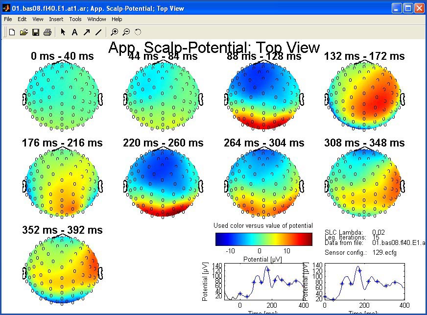Figure 1: the default plot type of emegs3d: >>Plot2d<< layout, >>Sphere<< headmodel, >>autoscaled<<, with sensor positions indicated on all intervals, using 256 colors of the jet colormap, blue colors indicating low and red colors high amplitudes.

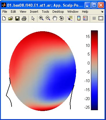
plot types:  emegs has 6 different plot layouts, that you can set using the Surf View- dropdownlist on the emegs3d-console: Spec. Surf. , All Surf I , All Surf II,  Plot2d,  Head View and Cols & Rows.

Figure 2: Surf View, Head View and Render Model controls

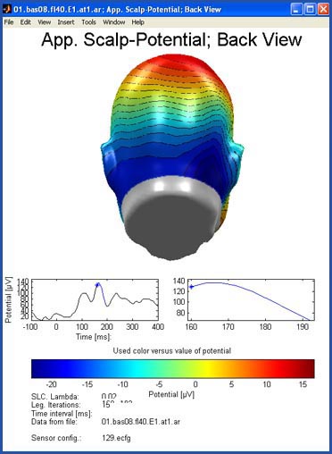
Spec. Surf. , All Surf I , All Surf II and  Head View will print only one time point, Plot2d and Cols & Rows display an interval sequence. Spec. Surf. , All Surf I , All Surf II will give additional views and information, Head View shows only the surface model with an amplitude colorbar.This sequence is taken from the emegs3d-console as described at interval settings.  [Top]

Spec. Surf.
All   Surf I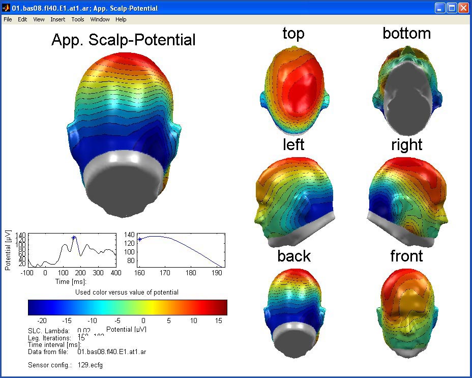
All Surf II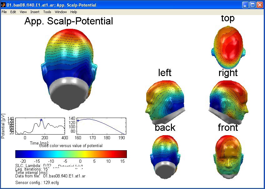
Plot2d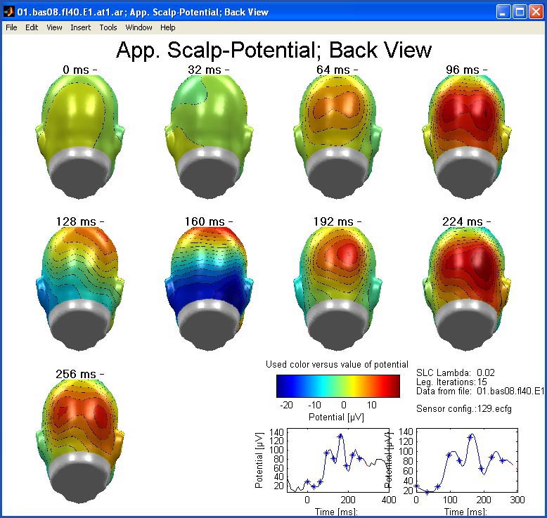
HeadView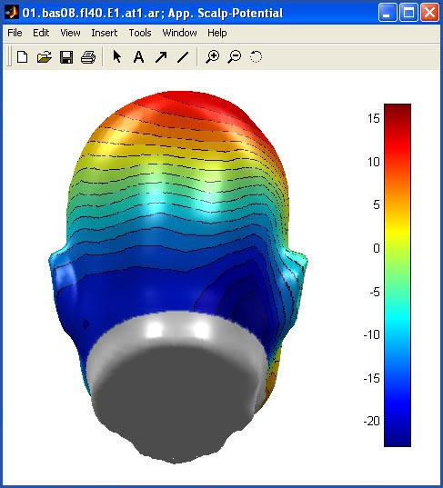
Cols&Rows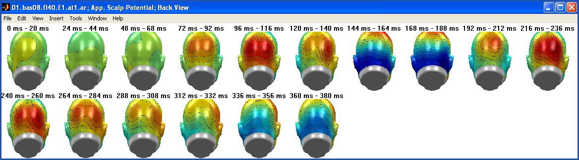
Figure 3: plot layouts, set using the Surf View dropdownlist.

head orientation:   you can select the initial position of the camera relative to the headmodel using the Head View - dropdownlist on the emegs3d-console. Some head models can later be turned to see a different side, but not all. If the six options (top, bottom, left, right, front, back) are too rough, you can use the theta and phi edit boxes to enter azimuth and elevation angles parametrically. Note that these angles are standard matlab spherical coordinates, unlike the sensor coordinates used by emegs.

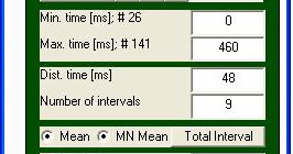
Figure 4: Min. time, Max. time, Dist. time, Number of intervals, Total Interval and Mean/MN Mean controls

interval settings:  interval definitions on the emegs3d-console are set using the controls shown above: the time range from Min. time [ms] to Max. time [ms]  is divided into Number of intervals segments, that each are of length Dist. time [ms]. You can change any of these values, and emegs will try to adjust the others accordingly.  If a segment covers more than 1 datapoint, the plotted data is calculated as average over the points of the segment, as indicated by the Mean - radiobutton. If this button is not activated, not the average is taken, but simple the first data point in the segment.  To cover the total available interval with segments of mimimum duration and thus avoid any averaging, you can use the Total Interval - button.  [Top]

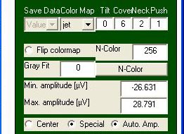
Figure 5: Color Map, Flip colormap, N-Color, Min. amplitude, Max. amplitude, Center, Special and Auto. Amp. controls

amplitude scaling:   the default behavior of emegs is to scale each plot automatically in such a way, that the entire range of colors of the present colormap are used.  This is indicated by the Auto. Amp. - radiobutton, which should be deactivated, if you wish to set the color limits manually with the Min. amplitude - and Max. amplitude - editboxes. The autoscaling is in fact often misleading, as event the smallest differences will be scaled to cover the entire range of available colors. When comparing experimental conditions, it is therefore advisable to first create a plot using the autoscaling to get a realistic scaling range, but then to deactivate it when creating plot for the different conditions.
Jet is the standard colormap of emegs, thus low amplitudes will be colored in blue, high amplitudes in red, but you can change the colormap type by selecting a differnt matlab color map in the Color Map- dropdownlist. You can change the orientation of the colormap using the Flip colormap - radiobutton and set the colormap resolution using the N-Color -editbox. Low resolution will result in areas of the same color, whereas high resolution will result in smooth color gradients.  [Top]

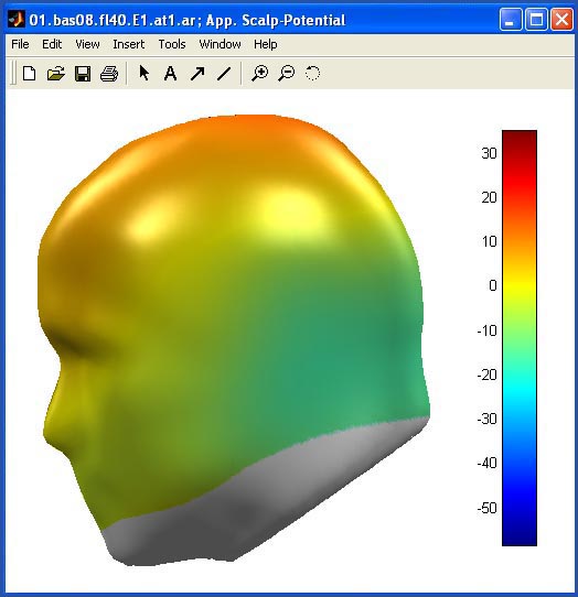
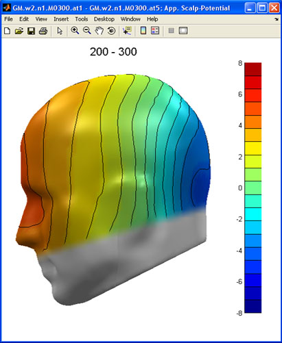
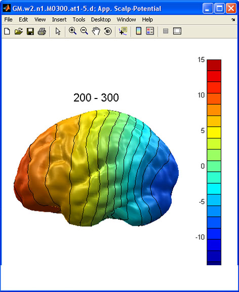
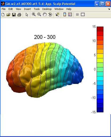
render models:  emegs offers a number of surface models, that evoked brain activity signal can be projected on. Examples of each are given below using the HeadView plot layout seen from the left side.  Please note, that no inference about brain activity is made with any model. All models are simply surface models, that a given evoked activity is mapped on. This activity can be dipole activity, but does not have to be - although the brain models obviously are meant for diplaying dipole activations. To make estimations about generating brain areas, see the source localization & synthetic data - section.  [Top]

Sphere		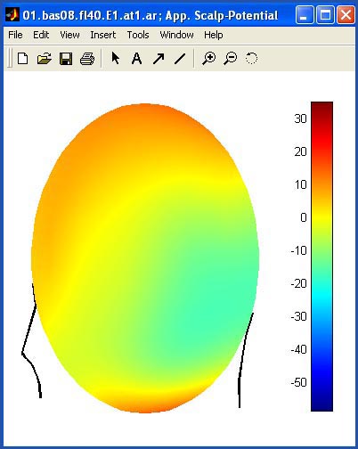		Head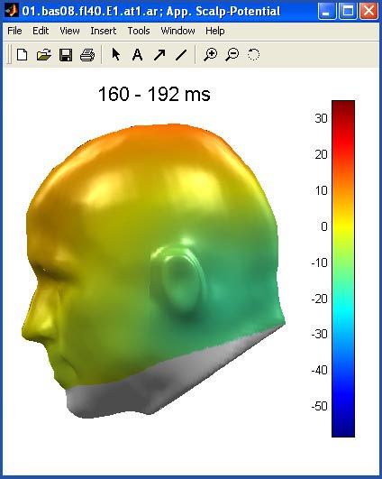
Head Smooth				Brain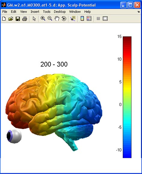
Brain Low Smoothing		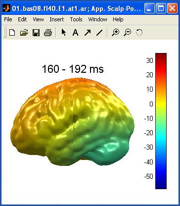		Brain High Smoothing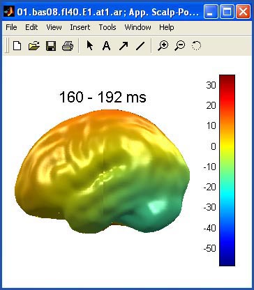
BrainNC Low Smoothing		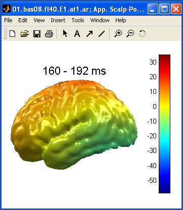		BrainNC High Smoothing
Head Neck		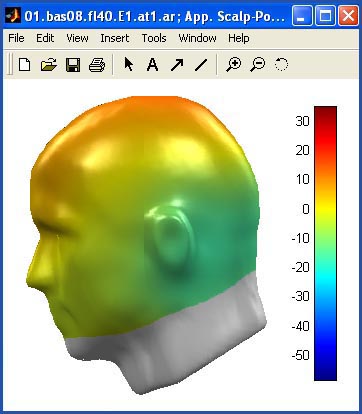		Head Vol  (enhanced contour line rendering)
BrainVol (enhanced contour line rendering)				BrainNCVol (enhanced contour line rendering)
Brain (HighRes)
Figure 6: Render models, set using the Render model control.

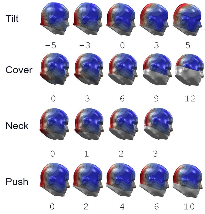
texture mapping:   the render models head, head smooth, brain low smoothing, brain high smoothing, brainnc low smoothing, brainnc high smoothing and head neck employ texture mapping to display the signal topography on the render model. This means that first a jpg image file is created (the texture, saved in .../emegs2.1/contourplottmp.jpg) which is then pulled like a glove over (mapped to) the headmodel:. You can influence this mapping using the Tilt, Cover, Neck and Push editboxes shown in figure 5. The effect of each is shown on the examples below: Tilt will rotate the potential map around the X-Axis (see sensor cofigurations), positive values forward, negative values backward. Be sure to activate leadfield recalculation for every plot if you change the Tilt value. Cover will cover increasing amount of the potential map with white pixels, hiding the original colors. Neck selectively covers area on the back, leaving the front part unchanged. Push adds additional white area on the bottom, pushing the potential map higher, without hiding any parts of it.  [Top]

Figure 7: Sensors, Contour, Latency & PotCont controls

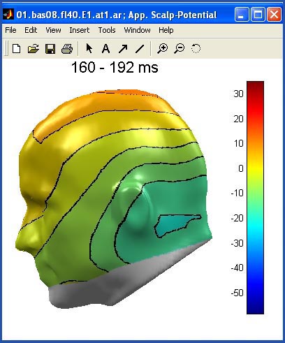
contour lines:   some of the shown render models offer the possibilty to display activity as a smooth color gradients or as contoured areas of the same color. This is done using the PotCont- dropdownlist. Using the head model, the contour options are illustrated in the following table: [Top]

Smooth		Contour		WContour		2Contour		2WContour
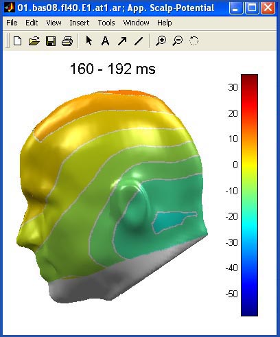Figure 8: contour line options, set using the PoCont control.

sensor type, color and size:   sensor position markers can be activated using the Sensors- dropdownlist. For a sequence, this can be done only for the first plot in the sequence or for all intervals. The marker type can be set using emegs3d-style-menu: as text, on the texture or as cylinder. The three types  are illustrated below (click to enlarge). As the activity for the here used 'Head' render model is mapped as a texture, the texture type is the precicest concerning it's correspondence with the activity. For this render model, the texture type should be used to check wether the texture position, the neck coverage and the texture size is adequate for your sensor configuration. The cylinder sensor type can be adjusted in color and object size using the emegs3d-style-menu (\Style\Sensor size  and \Style\Sensor color). [Top]

Text		Texture		Cylinder
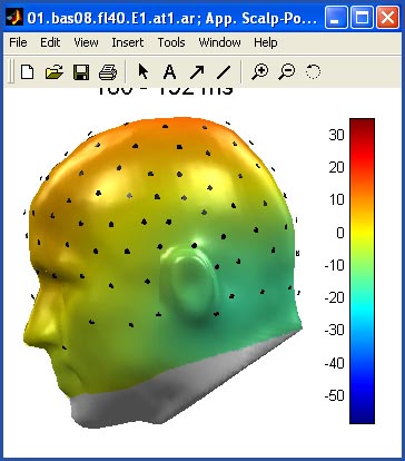Figure 8: contour line options, set using the PoCont control.

latency:   latency information can be activated using the Latency- dropdownlist. For a sequence, this can be done only for the first plot in the sequence or for all intervals. [Top]

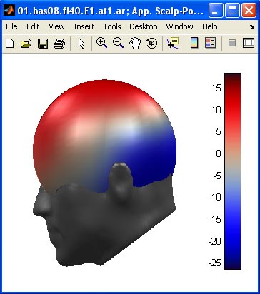
sphere model head shape:   Although artificial in appearance, the sphere model is closest to the actual data and all 3d projections are calculated based on the spherical head model. However, with only the sphere visible, it is hard to distinguish left from right and front from back. This is made a lot easier when additional shapes are displayed for the nose, the ears and the neck. The default setting is that these are displayed as line plots, but you can select also a 3d contour type from the Contour-dropdownlist shown in figure 7.You can select the transparency of this 3d object using the emegs3d-style menu (\Style\3d contour alpha\).  Samples of line and 3d contours are given below. [Top]

line contour		3d contour (alpha = 1)		3d contour (alpha = 0.2)
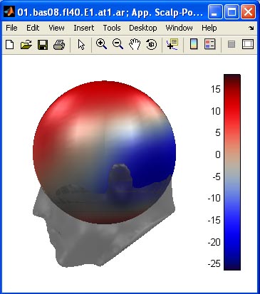Figure 8: head shape options, set using the Contour control.